Open in Google Colab
Run this exact tutorial interactively in Google Colab
Simulating Population Shift to Expose Model Drift in Life Insurance Underwriting
If you trained an underwriting model on a 2015 applicant population, what happens when the 2026 population looks meaningfully different? This tutorial shows how to use DataFramer to create that shifted population on purpose, then run a frozen underwriting model against both groups to see whether the score distribution has drifted.Key finding: when scored against the shifted 2026 population — older applicants, higher BMI, more medical conditions — the frozen 2015 model classified 37.8 percentage points fewer applicants as high-risk (classes 7–8), and the mean raw score dropped from 5.6 to 4.4. The model looked at a sicker population and concluded it was safer. This is the shape of silent model drift: nothing looks broken, scores are produced, policies are issued, and the financial exposure only becomes visible in claims data months or years later.You will walk through the same stages as the notebook:
- Train a simple life-insurance risk model on the Prudential underwriting dataset.
- Train a frozen 2015 underwriting model and learn the class thresholds that define its 2015 calibration.
- Profile the 2015 applicant population as the model’s baseline environment.
- Use DataFramer to build a Specification from the 2015 population and shift it to simulate a 2026 applicant pool.
- Generate the shifted 2026 synthetic population.
- Score both populations with the unchanged 2015 model and compare the risk distributions.
- Frame the business question the model cannot answer on its own.
Prerequisites
- Python 3.9+
- A
DATAFRAMER_API_KEY train.csvfrom the Prudential underwriting dataset placed in a localfiles/directory
Part 1: Train the Frozen 2015 Underwriting Model
The notebook starts from Prudential underwriting data with 128 columns. To stay within DataFramer’s seed limits while preserving enough underwriting signal, it selects 29 original fields and adds one derived feature:- Biometrics such as
Ins_Age,Ht,Wt, andBMI(all normalized to [0, 1]) - Product attributes from
Product_Info_* - Employment and insured profile variables
- Insurance and family history variables
Medical_History_1Med_Keywords_Count, which aggregates the 48 binaryMedical_Keyword_*columns into a single countResponse, the underwriter-assigned risk class from 1 to 8
XGBRegressor. Instead of predicting the 1–8 risk classes directly, it predicts a continuous score and then learns seven thresholds that map that score back onto Prudential’s eight underwriting classes. Those thresholds are optimized by maximizing quadratic weighted kappa (QWK) via Nelder-Mead.
Part 2: Establish the 2015 Calibration
The notebook trains anXGBRegressor on the selected features, then learns seven class thresholds that map the model’s continuous score back to Prudential’s 8-level underwriting scale.
Those thresholds are calibrated on the 2015 training population and then held fixed for the rest of the analysis. That frozen threshold set is the 2015 calibration.
Part 3: Profile the 2015 Applicant Population
Before simulating drift, score the original applicant population with the frozen model and record the baseline distribution of predicted underwriting classes.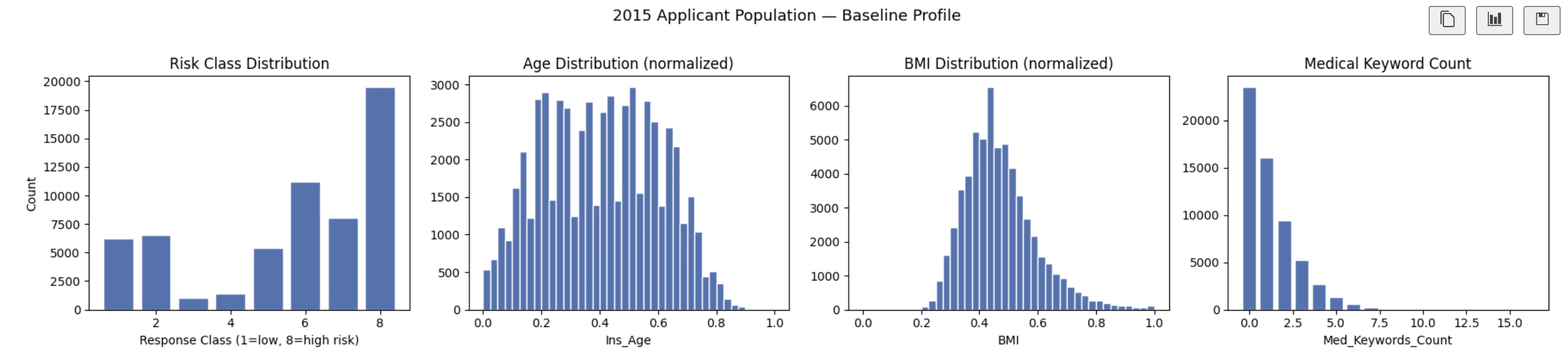
Part 4: Build and Shift a DataFramer Specification
Build the spec from the 2015 population
Upload the full 2015 applicant table as a seed dataset. DataFramer analyzes the schema, value ranges, and inter-feature relationships, then produces a Specification that captures the population in a reusable form.Shift the spec to simulate a 2026 population
The tutorial edits the spec to represent three directional changes in the applicant pool:Ins_Age: increase the mean by 7 yearsBMI: increase the mean by 9%Med_Keywords_Count: increase the mean by 50%
base_distributions inside the spec and writes the updated YAML back to DataFramer:
Part 5: Generate the Shifted Population
With the updated spec in place, generate a synthetic population of 500 applicants: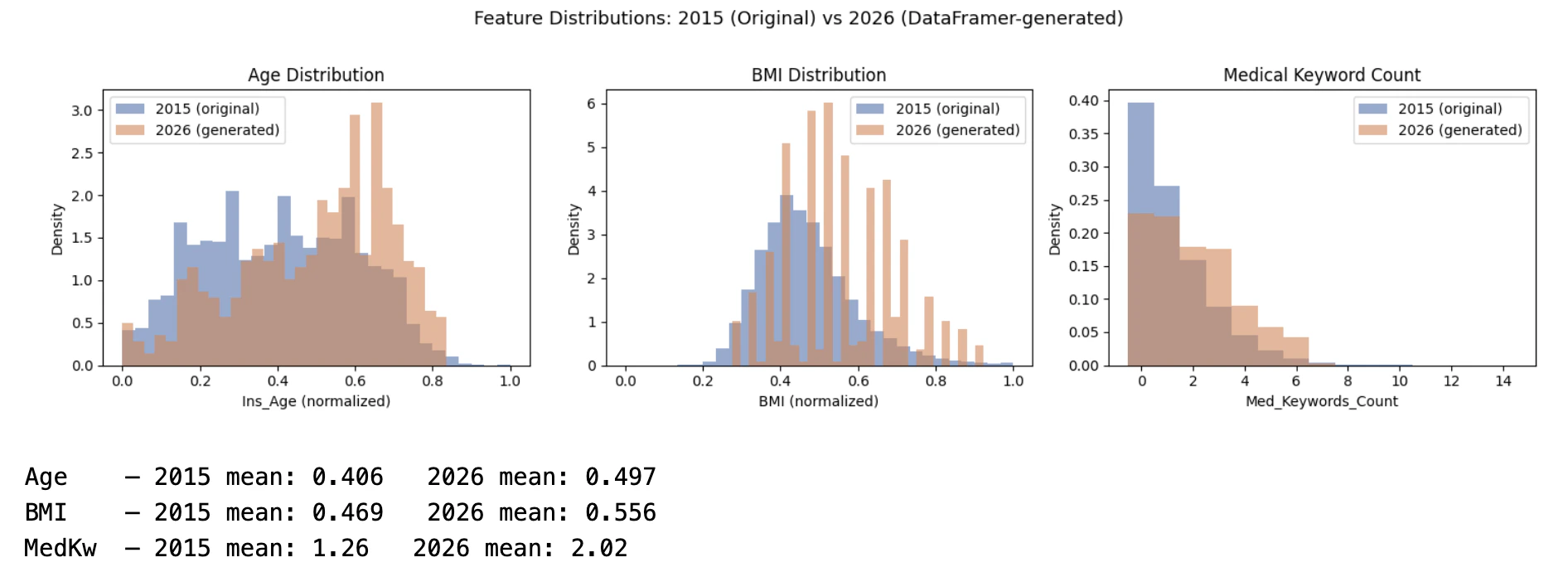
Part 6: Score Both Populations with the Same 2015 Calibration
Now apply the unchanged model and unchanged thresholds to both populations:- Risk-class percentages for classes 1 through 8
- The share of applicants landing in high-risk classes 7 and 8
- The full raw score distributions under the fixed 2015 thresholds
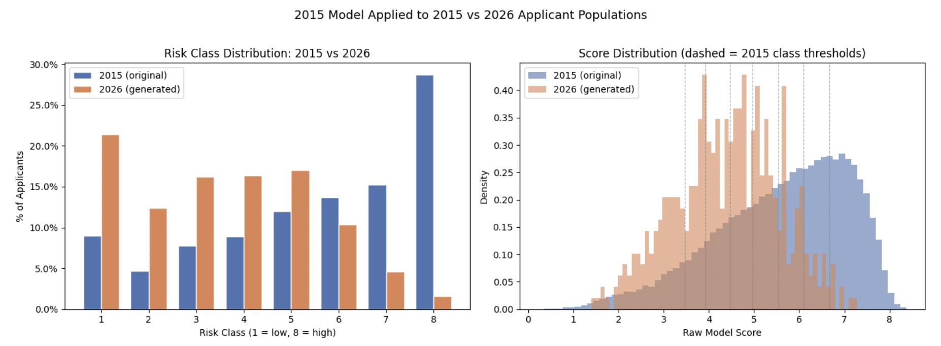
The Business Question the Model Cannot Answer on Its Own
This is the key business takeaway from the notebook. The frozen 2015 model, with the same weights and the same class thresholds, classified 37.8 percentage points fewer applicants from the shifted 2026 population as high-risk (classes 7–8). The mean raw score dropped from 5.6 to 4.4. The model looked at a population that is older, heavier, and carries more medical conditions — and concluded it was safer. There are two plausible explanations:- The 2015 weights no longer reflect reality. A feature that was rare and strongly correlated with mortality risk in 2015 may now be common and well-managed. The model still applies the 2015 coefficient to a signal that has lost its predictive content, systematically underpricing risk for exactly the applicants who pose the greatest exposure.
- The model is extrapolating outside its training regime. The 2015 training set never saw enough applicants with this specific combination of age, BMI, and keyword count. When pushed outside its training distribution, the model collapses toward the center — producing lower predicted risk scores precisely where the uncertainty is highest.
What DataFramer Enables Here
- Create a realistic shifted underwriting population without exposing real policyholder data
- Control which applicant characteristics move and by how much
- Re-run the same drift scenario against multiple model versions or calibration strategies
- Reproduce the scenario reliably across model versions or underwriting rules
- Do the analysis in hours instead of waiting months for naturally accumulated data with the right distribution
Related Tutorials
Financial Document QA Eval
Build custom eval sets and stress-test extraction quality on synthetic edge-case PDFs
Support Chatbot Broader Evals
Generate broader contextual evaluation sets with golden responses